Geometric Distribution Calculator

Get Homework Help

The Geometric Distribution is a key concept in probability theory, used to model the number of trials needed to achieve the first success in a sequence of independent trials. The Geometric Distribution Calculator for a Table simplifies these calculations, making it easy to compute probabilities and expectations for various datasets. Whether you’re a student, researcher, or data analyst, this tool is your go-to solution for geometric probability problems.

1. Introduction to the Geometric Distribution Calculator

The Geometric Distribution applies to scenarios where you’re interested in the number of trials required to achieve the first success. It’s widely used in quality control, reliability analysis, and even gaming probabilities.

Our Geometric Distribution Calculator supports tabular data, allowing you to analyze multiple scenarios in seconds. From predicting the likelihood of success in experiments to analyzing customer behavior, this tool is indispensable for probability analysis.

2. What is the Formulae used?

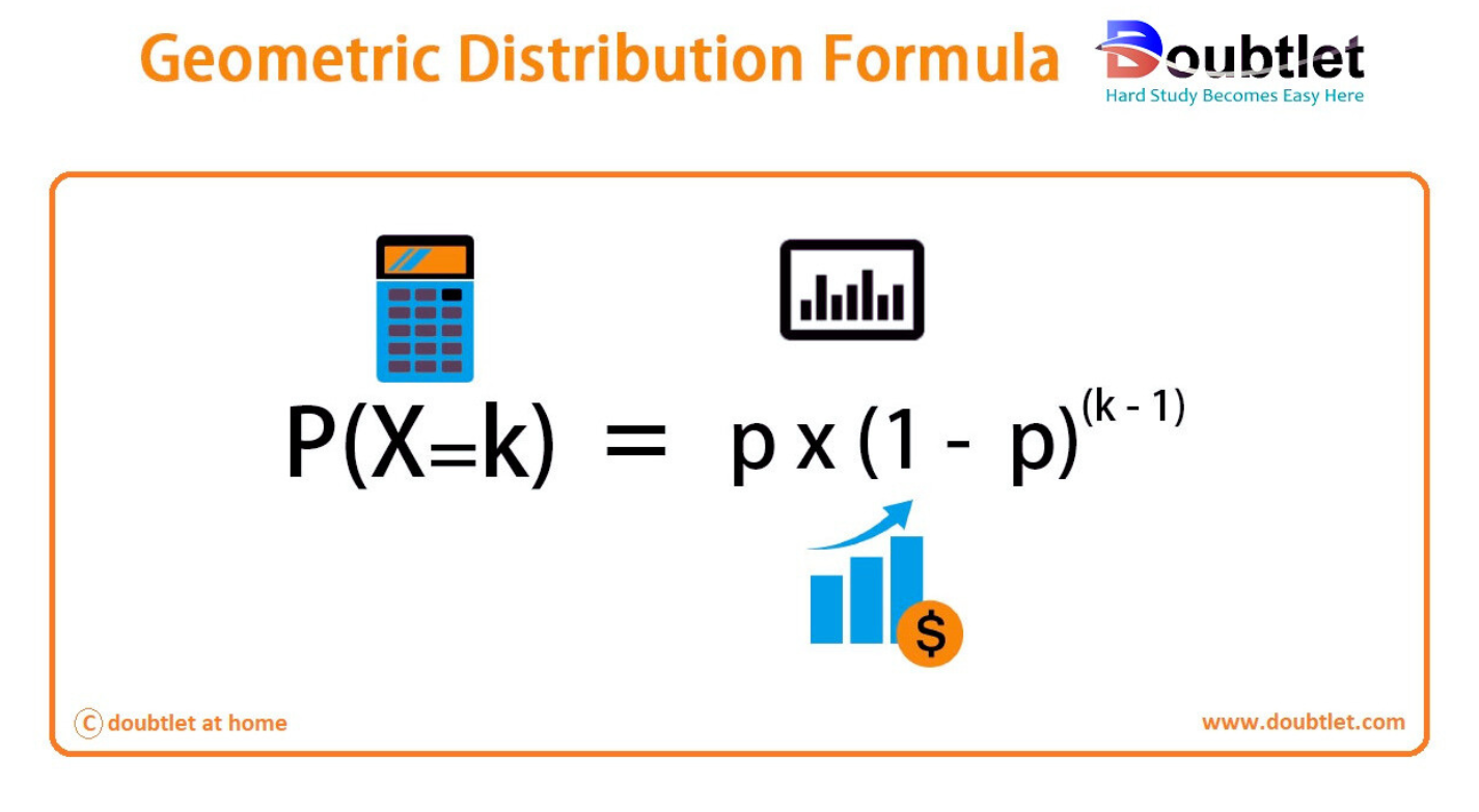
The Probability Mass Function (PMF) for the Geometric Distribution is:

$P(X = k) = (1 - p)^{k-1} \cdot p$

Where:

• $P(X = k)$: Probability of the first success occurring on the $k$-th trial.
• $p$: Probability of success in a single trial.
• $1 - p$: Probability of failure in a single trial.
• $k$: Trial number where the first success occurs $(k = 1, 2, 3, \dots)$.

Cumulative Probability (CDF):

The cumulative probability is:

$P(X \leq k) = 1 - (1 - p)^k$

Mean $(\mu)$:

$\mu = \dfrac{1}{p}$

Variance $(\sigma^2)$:

$\sigma^2 = \dfrac{1 - p}{p^2}$

These formulas allow for a detailed analysis of probabilities and expectations in the Geometric Distribution.

Geometric Distribution Formula

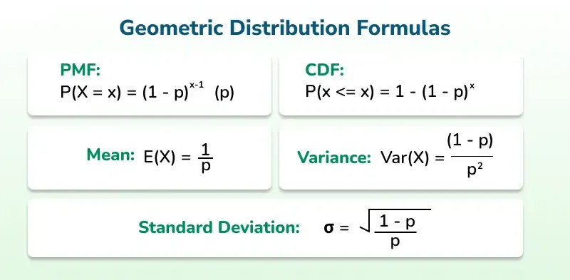
There are two geometric probability formulas:

• Geometric distribution PMF:

  $P(X = x) = (1 - p)^{x-1} \cdot p$

• Geometric distribution CDF:

  $P(X \leq x) = 1 - (1 - p)^x$

A geometric distribution can be described by both the probability mass function (PMF) and the cumulative distribution function (CDF). The probability of success of a trial is denoted by $p$, and failure is given by $q$, where $q = 1 - p$.

A discrete random variable, $X$, that has a geometric probability distribution is represented as:

$X \sim G(p)$

Geometric Distribution PMF

The probability mass function can be defined as the probability that a discrete random variable, $X$, will be exactly equal to some value, $x$. The formula for the geometric distribution PMF is given as follows:

$P(X = x) = (1 - p)^{x-1} \cdot p$

where $0 < p \leq 1$.

Geometric Distribution CDF

The cumulative distribution function (CDF) of a random variable, $X$, that is evaluated at a point, $x$, can be defined as the probability that $X$ will take a value that is less than or equal to $x$. It is also known as the distribution function.

The formula for the geometric distribution CDF is given as follows:

$P(X \leq x) = 1 - (1 - p)^x$

Geometric Distribution Mean (Expected Value)

The mean of the geometric distribution is also the expected value of the geometric distribution. The expected value of a random variable, $X$, can be defined as the weighted average of all values of $X$.

The formula for the mean of a geometric distribution is given as follows:

$E[X] = \dfrac{1}{p}$

Variance of Geometric Distribution

Variance can be defined as a measure of dispersion that checks how far the data in a distribution is spread out with respect to the mean.

The formula for the variance of a geometric distribution is given as follows:

$\text{Var}[X] = \dfrac{1 - p}{p^2}$

Standard Deviation of Geometric Distribution

The standard deviation can be defined as the square root of the variance. The standard deviation also gives the deviation of the distribution with respect to the mean.

The formula for the standard deviation of a geometric distribution is as follows:

$\text{S.D.} = \sqrt{\text{Var}[X]}$

$\text{S.D.} = \dfrac{\sqrt{1 - p}}{p}$

3. How Do I Find the Geometric Distribution?

Steps to Calculate Manually:

1. Identify Parameters: Determine $p$ (probability of success) and $k$ (trial number).

2. Use the PMF: Substitute $p$ and $k$ into the formula:

   $P(X = k) = (1 - p)^{k-1} \cdot p$

3. Compute Cumulative Probability (if needed): Use:

   $P(X \leq k) = 1 - (1 - p)^k$

4. Calculate Mean and Variance (if required): Use the formulas for $\mu$ and $\sigma^2$.

Example:

Problem: A basketball player has a $30$% chance of making a free throw $(p = 0.3)$. What’s the probability they succeed on the $4$th attempt?

1. PMF for $P(X = 4)$:

$P(X = 4) = (1 - 0.3)^{4-1} \cdot 0.3$

$P(X = 4) = 0.7^3 \cdot 0.3$

$P(X = 4) = 0.1029$

Answer: The probability of success on the 4th attempt is approximately $P(X = 4) = 0.1029$.

Note: Manually solving for large datasets can be cumbersome, but our calculator simplifies these calculations.

Overview of Geometric Distribution

The Geometric Distribution models the number of trials until the first success in a sequence of independent Bernoulli trials (success or failure).

• PMF (Probability Mass Function):

$P(X = k) = (1 - p)^{k-1} \cdot p, \quad k = 1, 2, 3, \ldots$

Where:

• $p$: Probability of success in each trial.

• $k$: The trial on which the first success occurs.

• Mean $(\mu)$:

$\mu = \dfrac{1}{p}$

• Variance $(\sigma^2)$:

$\sigma^2 = \dfrac{1 - p}{p^2}$

Example 1: First Success in Customer Service

The probability of successfully resolving a customer’s issue on a single call is $p = 0.3$.
What is the probability that:

1. The first success occurs on the $3$rd call $(P(X = 3))$?
2. The first success occurs within the first $5$ calls $(P(X \leq 5))$?

Solution:

1. Probability of First Success on $3$rd Call $(P(X = 3))$

Use the PMF formula:

$P(X = k) = (1 - p)^{k-1} \cdot p$

Substitute $k = 3$ and $p = 0.3$:

$P(X = 3) = (1 - 0.3)^{3-1} \cdot 0.3 = (0.7)^2 \cdot 0.3 = 0.49 \cdot 0.3 = 0.147$

2. Probability of First Success Within the First $5$ Calls $(P(X \leq 5))$

Use the CDF (Cumulative Distribution Function):

$P(X \leq k) = 1 - (1 - p)^k$

Substitute $k = 5$ and $p = 0.3$:

$P(X \leq 5) = 1 - (1 - 0.3)^5 = 1 - (0.7)^5$

$P(X \leq 5) = 1 - 0.16807 = 0.83193$

Answer:

• $P(X = 3) = 0.147$
• $P(X \leq 5) \approx 0.83193$

Example 2: Quality Control

In a factory, the probability of producing a defective item is $p = 0.1$.
What is the probability that:

1. The first defective item is found on the $4$th inspection $(P(X = 4))$?
2. The first defective item is found after the $6$th inspection $(P(X > 6))$?

Solution:

1. Probability of First Defect on $4$th Inspection $(P(X = 4))$

Use the PMF formula:

$P(X = k) = (1 - p)^{k-1} \cdot p$

Substitute $k = 4$ and $p = 0.1$:

$P(X = 4) = (1 - 0.1)^{4-1} \cdot 0.1 = (0.9)^3 \cdot 0.1$

$P(X = 4) = 0.729 \cdot 0.1 = 0.0729$

2. Probability of First Defect After the 6th Inspection $(P(X > 6))$

Use the complement rule:

$P(X > k) = (1 - p)^k$

Substitute $k = 6$ and $p = 0.1$:

$P(X > 6) = (1 - 0.1)^6 = (0.9)^6$

$P(X > 6) = 0.531441$

Answer:

• $P(X = 4) = 0.0729$
• $P(X > 6) = 0.5314$

Graph of Geometric Distribution

Let’s plot the PMF for a Geometric Distribution with $p=3$ (e.g., customer service example).

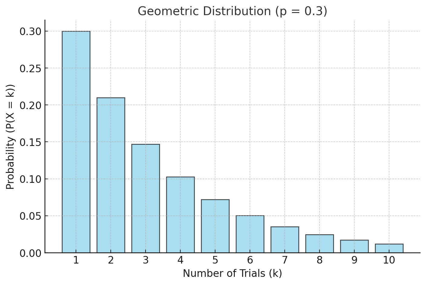
Explanation of the Geometric Distribution Graph:

1. X-Axis $(k)$: Represents the number of trials until the first success.
2. Y-Axis $(P(X = k))$: Represents the probability of the first success occurring on trial $k$.
3. Shape of the Graph:
   • The probabilities decrease as $k$ increases because success is less likely as the trial count grows.
   • The highest probability is at $k = 1$ (success on the first trial).

For $p = 0.3$, the graph reflects that the likelihood of success decreases exponentially as the trial number increases.

Let me know if you have additional questions or need further clarification!

Example 1: Probability of First Success

A factory produces light bulbs, and $10$% of the bulbs are defective $(p = 0.1)$. What is the probability that the first defective bulb is found on:

1. The $4$th inspection $(P(X = 4))$?
2. At most the $3$rd inspection $(P(X \leq 3))$?
3. After the $5$th inspection $(P(X > 5))$?

Solution:

1. $P(X = 4)$: Use the PMF formula:

   $P(X = k) = (1 - p)^{k-1} \cdot p$

   Substitute $k = 4$ and $p = 0.1$:

   $P(X = 4) = (1 - 0.1)^{4-1} \cdot 0.1 = (0.9)^3 \cdot 0.1$

   $P(X = 4) = 0.729 \cdot 0.1 = 0.0729$

2. $P(X \leq 3)$: Use the CDF formula:

   $P(X \leq k) = 1 - (1 - p)^k$

   Substitute $k = 3$ and $p = 0.1$:

   $P(X \leq 3) = 1 - (1 - 0.1)^3 = 1 - (0.9)^3$

   $P(X \leq 3) = 1 - 0.729 = 0.271$

3. $P(X > 5)$: Use the complement rule:

   $P(X > k) = (1 - p)^k$

   Substitute $k = 5$ and $p = 0.1$:

   $P(X > 5) = (1 - 0.1)^5 = (0.9)^5$

   $P(X > 5) = 0.59049$

Example 2: Time to First Success

A basketball player has a $60$% chance $(p = 0.6)$ of making a free throw. Find:

1. The probability that the player makes their first basket on the $2$nd attempt.
2. The probability that the player makes their first basket within the first $4$ attempts.
3. The probability that the player misses the first $5$ attempts.

Solution:

1. $P(X = 2)$:

   $P(X = 2) = (1 - p)^{2-1} \cdot p = (1 - 0.6)^1 \cdot 0.6 = 0.4 \cdot 0.6 = 0.24$

2. $P(X \leq 4)$:

   $P(X \leq k) = 1 - (1 - p)^k$

   Substitute $k = 4$ and $p = 0.6$:

   $P(X \leq 4) = 1 - (1 - 0.6)^4 = 1 - (0.4)^4$

   $P(X \leq 4) = 1 - 0.0256 = 0.9744$

3. $P(X > 5)$:

   $P(X > k) = (1 - p)^k$

   Substitute $k = 5$ and $p = 0.6$:

   $P(X > 5) = (1 - 0.6)^5 = (0.4)^5$

   $P(X > 5) = 0.01024$

Graph of Geometric Distribution

Let’s plot the Geometric Distribution for $p=0.1$ (factory example).

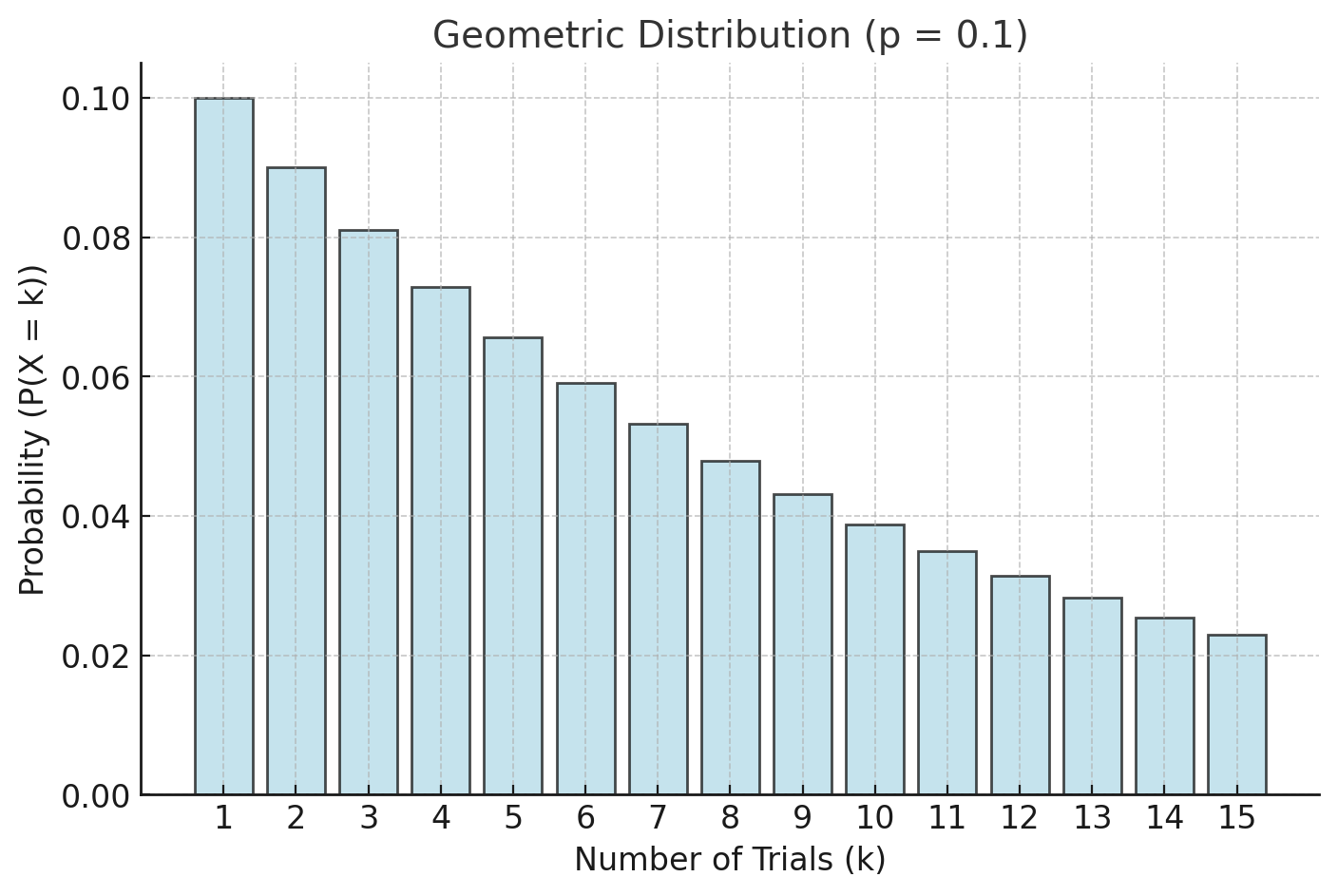
Explanation of the Geometric Distribution Graph:

1. X-Axis $(k)$: Represents the number of trials until the first success.

2. Y-Axis $(P(X = k))$: Represents the probability of achieving the first success on trial $k$.

3. Shape of the Graph:

   • The probabilities decrease as $k$ increases.
   • The highest probability is for $k = 1$, where success occurs on the first trial.

For $p = 0.1$, the graph shows a sharp decrease, indicating that success is more likely to occur earlier in the trials.

Summary of Examples:

4. Why Choose Our Geometric Distribution Calculator?

$\bold{Easy \space \space to \space Use}$
Our calculator page provides a user-friendly interface that makes it accessible to both students and professionals. You can quickly input your square matrix and obtain the matrix of minors within a fraction of a second.

$\bold{Time \space Saving \space By \space automation}$
Our calculator saves you valuable time and effort. You no longer need to manually calculate each cofactor, making complex matrix operations more efficient.

$\bold{Accuracy \space and \space Precision}$
Our calculator ensures accurate results by performing calculations based on established mathematical formulas and algorithms. It eliminates the possibility of human error associated with manual calculations.

$\bold{Versatility}$
Our calculator can handle all input values like integers, fractions, or any real number.

$\bold{Complementary \space Resources}$
Alongside this calculator, our website offers additional calculators related to Pre-algebra, Algebra, Precalculus, Calculus, Coordinate geometry, Linear algebra, Chemistry, Physics, and various algebraic operations. These calculators can further enhance your understanding and proficiency.

5. A video based on how to Evaluate the Geometric Distribution.

6. How to use this calculator?

Using the Geometric Distribution Calculator is straightforward:

1. Input Data: Enter the probability of success $(p)$ and the trial number $(k)$.

2. Choose Output: Select individual probabilities, cumulative probabilities, or both.

3. Click Calculate: Instantly view the results along with intermediate steps.

This calculator removes the complexity, letting you focus on interpreting the results.

7. Solved Examples on Geometric Distribution

Example 1:

A software tester has a $25$% chance $(p = 0.25)$ of finding a bug in a test. What’s the probability they find the first bug on the $5$th test?

Solution:

1. PMF for $P(X = 5)$:

   $P(X = 5) = (1 - 0.25)^{5-1} \cdot 0.25 = 0.75^4 \cdot 0.25 = 0.0791$

Example 2: Tabular Data:

Steps:

1. Input each row into the calculator.

2. Compute probabilities for each combination of $p$ and $k$.

Our calculator handles these calculations effortlessly, even for extensive datasets.

8. Frequently Asked Questions (FAQs)

Q1. What is the Geometric Distribution?

It models the probability of the first success occurring on the $k$-th trial in a series of independent trials with a constant success probability.

Q2. What is $p$ in the formula?

$p$ represents the probability of success in a single trial.

Q3. Is this calculator free to use?

Yes, our Geometric Distribution Calculator is completely free.

Q4. Does it handle large datasets?

Yes, it supports extensive tabular data.

Q5. Can I calculate cumulative probabilities?

Yes, the calculator provides both individual and cumulative probabilities.

Q6. Is the calculator mobile-compatible?

Absolutely, it works seamlessly on all devices.

Q7. Can I export results?

Yes, outputs can be downloaded for further analysis.

Q8. Does it show intermediate steps?

Yes, detailed calculations are displayed for better understanding.

9. What are the real-life applications?

The Geometric Distribution is widely used across various fields:

• Quality Control: Model the number of inspections needed to detect a defect.
• Education: Analyze quiz or test retake probabilities.
• Healthcare: Study the likelihood of treatment success over time.
• Sports: Predict the number of attempts needed for success in games.
• Customer Service: Estimate the number of calls required to resolve an issue.

Fictional Anecdote: Mark, a software engineer, uses our Geometric Distribution Calculator to predict the number of tests needed to uncover a critical bug. With accurate insights, he optimizes testing strategies, reducing development time by 15%.

10. Conclusion

The Geometric Distribution Calculator is an essential tool for anyone working with probability scenarios. It simplifies calculations, ensures accuracy, and saves time, making it ideal for professionals, students, and researchers alike.

Ready to analyze probabilities like a pro? Try our Geometric Distribution Calculator today and unlock the power of precision!

---

If you have any suggestions regarding the improvement of the content of this page, please write to me at My Official Email Address: doubt@doubtlet.com

$\fcolorbox{black}{lightpink}{\color{blue}{Click here to Ask any Doubt}}$
Are you Stuck on homework, assignments, projects, quizzes, labs, midterms, or exams?
To get connected to our tutors in real time. Sign up and get registered with us.

$\color{red} \bold{Related \space Calculators}$
Binomial Distribution Calculator
Exponential Distribution Calculator
Margin of Error Calculator
Decimal to Percent calculator
Percent to Decimal calculator
Percent to Fraction calculator
Scientific Notation calculator